In epidemiological research, we often encounter situations where individuals experience the same event multiple times. Think of hospital readmissions, recurring infections, or repeated disease flare-ups. Analyzing this type of data requires specialized statistical approaches that go beyond traditional survival analysis, which typically focuses only on the time to the first event.Amorim and Cai (2014) published a tutorial in the International Journal of Epidemiology that offers a comprehensive overview of different statistical models designed for recurrent event data. This blog post will walk you through the key concepts and models discussed in their paper, providing a framework for understanding and analyzing recurrent events in your own research.
Article Screenshot
Why Can’t We Just Use a Standard Survival Model?
The core issue with applying standard survival models, like the Cox proportional hazards model, to recurrent event data is the independence assumption. These models assume that each event is independent of the others. However, recurrent events within the same individual are inherently correlated. Ignoring this correlation can lead to:
Artificially narrow confidence intervals.
An inflated risk of falsely rejecting the null hypothesis.
Therefore, we need models that explicitly account for this within-individual correlation.
Modeling Approaches for Recurrent Event Data
Amorim and Cai (2014) outline five main modeling approaches for analyzing recurrent time-to-event data:
Andersen-Gill (AG) Model:
Concept: This model extends the Cox model by treating each event as a separate observation within the same individual. It uses a counting process framework, where the outcome of interest is the time since the study began until an event occurs (total time scale).
Key Assumption: The AG model assumes that any correlation between event times within a person can be explained by past events. In other words, time increments between events are conditionally uncorrelated, given the covariates.
When to Use: The AG model is appropriate when the dependence between subsequent events is mediated through time-varying covariates (e.g., number of previous events). It’s useful when you want to estimate the overall effect of factors on the intensity of recurrent events.
Example: Analyzing repeated occurrences of basal cell carcinoma, considering factors like sun exposure and previous treatments as time-varying covariates.
2. Prentice, Williams, and Peterson (PWP) Models:
Concept: PWP models analyze ordered multiple events by stratifying the data based on the prior number of events during the follow-up period.
Key Feature: The effect of covariates may vary from event to event in the stratified PWP models.
Types:
PWP-Total Time (TT): Evaluates the effect of a covariate for the kth event since the entry time in the study.
PWP-Gap Time (GT): Evaluates the effect of a covariate for the kth event since the time from the previous event. This approach resets the time index to zero after each recurrence, assuming a renewal process.
When to Use: PWP models are preferable when the effects of covariates are expected to differ across subsequent events. Gap time models are useful when events are infrequent or when you’re interested in predicting the next event.
Example: Studying viral infections, where the effect of vaccination might change with subsequent infections due to developing immunity.
3. Marginal Means/Rates Model:
Concept: This approach focuses on modeling the mean number of events or their occurrence rate.
Key Advantage: It does not require specifying dependence structures among recurrent event times within a subject.
When to Use: This model is useful when the dependence structure is complex, unknown, or not of primary interest. It provides a more flexible and parsimonious alternative to the AG model, especially when the dependence structure cannot be characterized by including time-varying covariates.
Example: Analyzing the accumulated cost of medical care, where the dependence between healthcare events might be complex and not easily captured by specific covariates.
4. Frailty Model:
Concept: This random-effects approach introduces a random covariate (the “frailty”) into the model to induce dependence among recurrent event times.
Key Idea: The frailty represents unmeasured heterogeneity between individuals that is not explained by observed covariates alone.
Common Implementation: Shared frailty model with random effects assumed to follow a gamma distribution.
When to Use: When there is heterogeneous susceptibility to the risk of recurrent events, and the differences between individuals are not captured by the measured covariates.
Example: Evaluating recurrent infections at the point of catheter insertion in dialysis patients, where some patients might be inherently more susceptible to infection due to unmeasured factors.
5. Multi-State Models (MSM):
Concept: MSM models explicitly define different states an individual can occupy and model the transitions between these states.
Application to Recurrent Events: In the context of recurrent events, the states can represent different stages of a disease or the occurrence of specific events.
Key Elements: Transition probabilities (probability of moving from one state to another) and transition intensities (instantaneous hazard of transitioning between states).
When to Use: MSMs are useful when you want to model the entire process of moving between different states, considering the history of events.
Example: Modeling hospitalizations and death in heart failure patients, where hospitalizations are recurrent events, and death is an absorbing state.
Choosing the Right Model
Selecting the appropriate model for your recurrent event data depends on several factors:
Number of events: The number of events per individual can influence the stability and reliability of model estimates.
Relationship between consecutive events: Consider whether events are independent, conditionally independent given covariates, or influenced by unmeasured factors.
Effects that may or may not vary across recurrences: Determine if the impact of covariates is consistent across all events or changes over time.
Biological process: The underlying biological mechanisms driving the recurrent events should inform your choice of model.
Dependence structure: Consider whether the dependence structure is of primary interest or a nuisance factor to be accounted for.
Research question: The specific question you are trying to answer will guide your model selection.
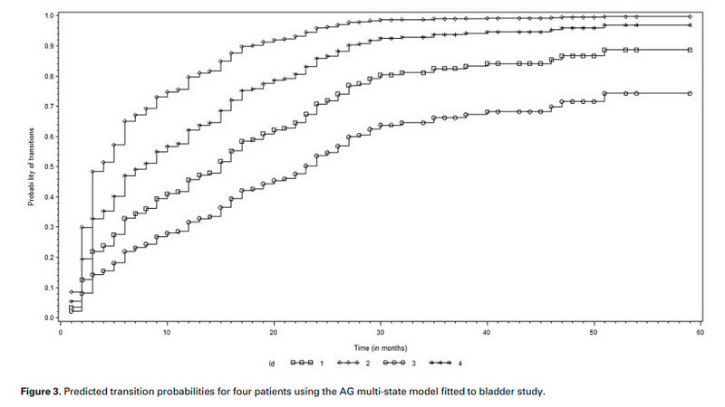
Predicted transition probabilities for four patients using the AG multi-state model fitted to bladder study
Conclusion
Analyzing recurrent event data requires careful consideration of the underlying assumptions and the specific research question. The models discussed by Amorim and Cai (2014) provide a valuable toolkit for epidemiologists and researchers in related fields. By understanding the strengths and limitations of each approach, you can choose the most appropriate model for your data and draw meaningful conclusions about the patterns and determinants of recurrent events.
Reference
Amorim, L. D. A. F., & Cai, J. (2015). Modelling recurrent events: a tutorial for analysis in epidemiology. International Journal of Epidemiology, 44(1), 324–333.